How to Make a Scatter Plot in Google Sheets?

When it comes to data visualization, Google Scatter Plots are less often used than other tools such as pie charts, line charts, and bar charts. Google sheets are a more convenient tool that comes with advanced features than the other ones. 

The crucial role of scatter plots is undeniable for data analysis, but if you think the tool is quite complex to master it and wonder how to make a scatter plot in Google Sheets?  here is the guide to help you create one. 

A Brief About Scatter Plots

Scatter Charts are a kind of graphical representation of the numerical coordination along the X and Y axis. It helps you to visualize various relationships that exist inside your data sets. It enables you to compare these data sets and aids to figure out how one variable is affected by the other. 

A scatter plot is very efficient as it can display the big picture of the data set. It shows the overall relationship and the trends that exist between the two variables.

Looking at the numbers alone is not particularly intuitive. It’s hard, impossible often, to determine how they’re related to each other.

In this guide, we will show you how to visualize the coordination between the data sets. 

How to Make a Scatter Plot in Google Sheets?

In the below example, the scatter plot demonstrates the relationship between the gold price in the respective months. As you can see, the price is continuously fluctuating, and the scatter plots show the trends. 

In general, the correlation can happen in two types. One, the variable in the x-axis is independent, and the variable in the y-axis is dependent. 

Second, the variables in both the X-axis and Y-axis are independent. Irrespective of the axis, the scatter plots can show the correlation between any two data sets. 

Step 1: Format your data

Create a new Google sheet from Google drive to start making the scatter plots. Start inserting your data in the sheets manually, or you can import the data. 

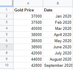
– Start entering the values for X-axis and give a column name. 

– Enter the values for Y-axis, which usually shows up as a series on the chart 

The Sample data set is shown in the below screen. 

Step 2: Create the Scatter Chart

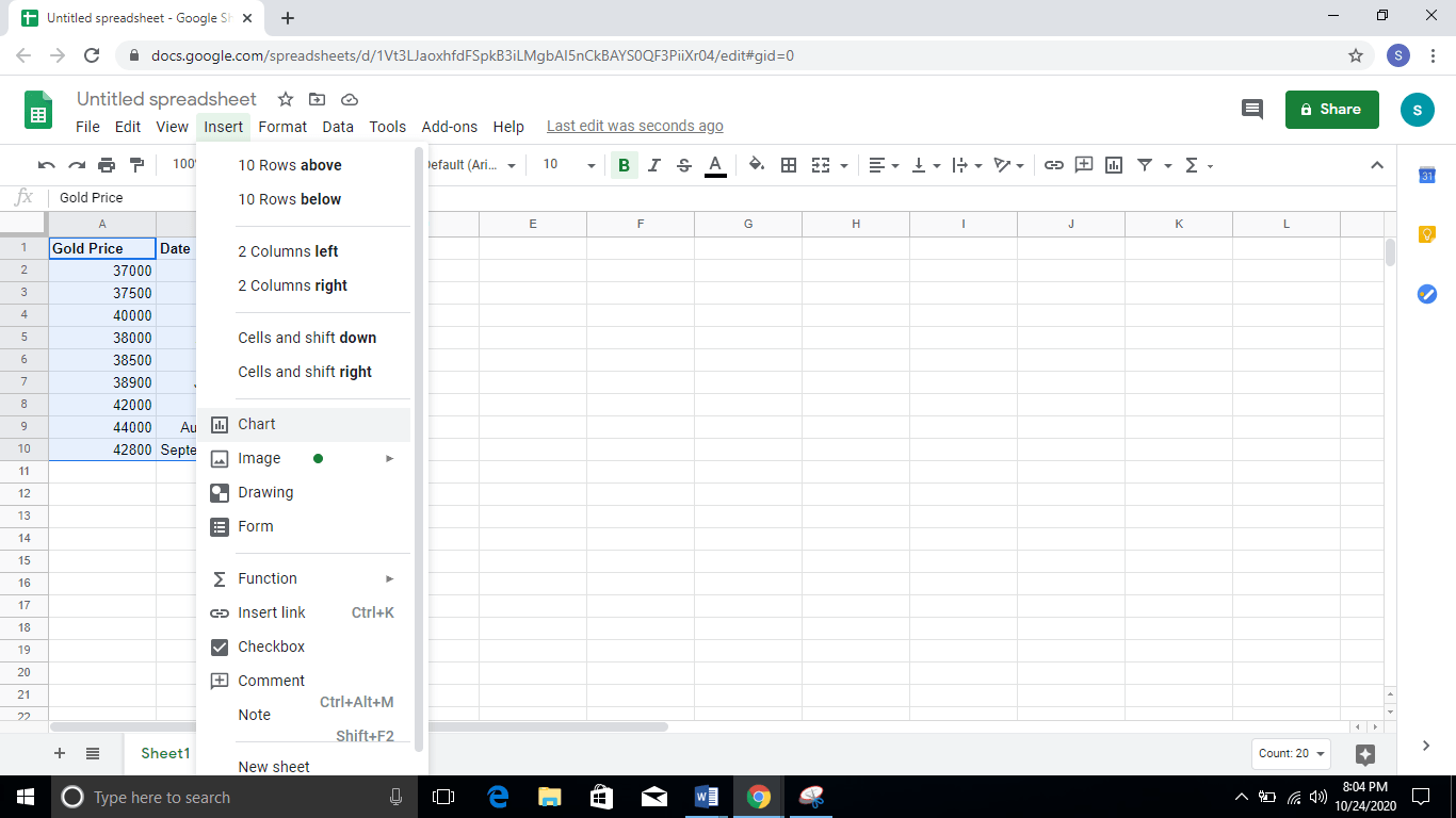
1. Once you enter the values, select the data range, and click on the Insert menu from the menu bar at the top. 
2. Select Chart option under Insert Menu. Your sheet will automatically generate the chart based on the data set entered.  You can see the Chart Editor on the right side of the sheet.
3. There are two tabs in the chart editor, Setup and Customize. Click on the Setup tab. Under Chart Type, click on the Scatter Chart. You will see the chart as shown in the below screen.
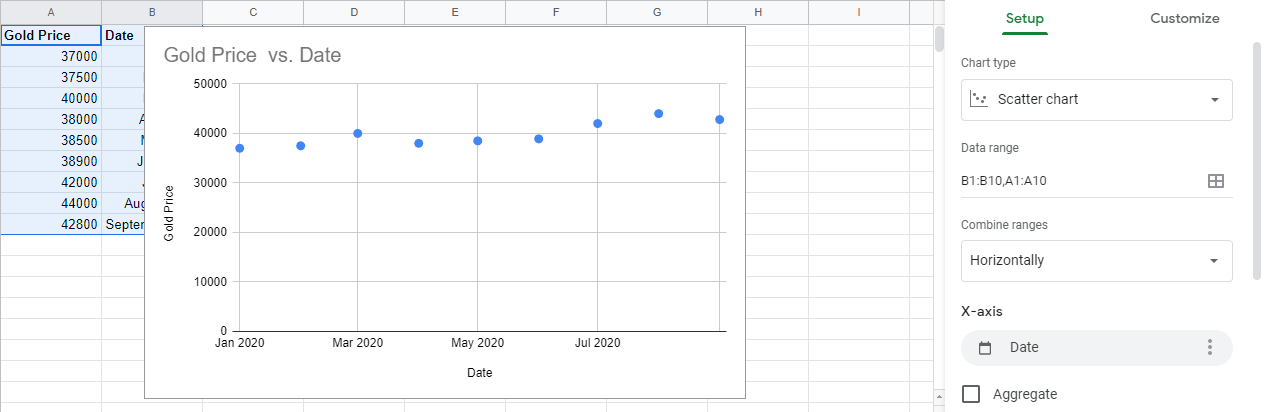
4. Scroll further in the Chart Editor to customize the chart design. 
5. Click on the check box beside the Aggregate option

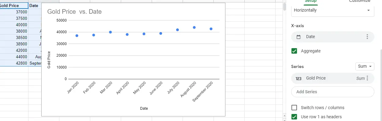
Now, your Scatter Plot is created. In the below steps you can learn how to customize the chart to make it more presentable. 

Step 3: Customize Scatter Plot

1. Click on the Customize tab under Chart Editor. You will see multiple options such as Series, Chart Style, Chart & Axis titles, Legends, and Vertical Axis. On clicking any of these options, the respective control panel will open up. 
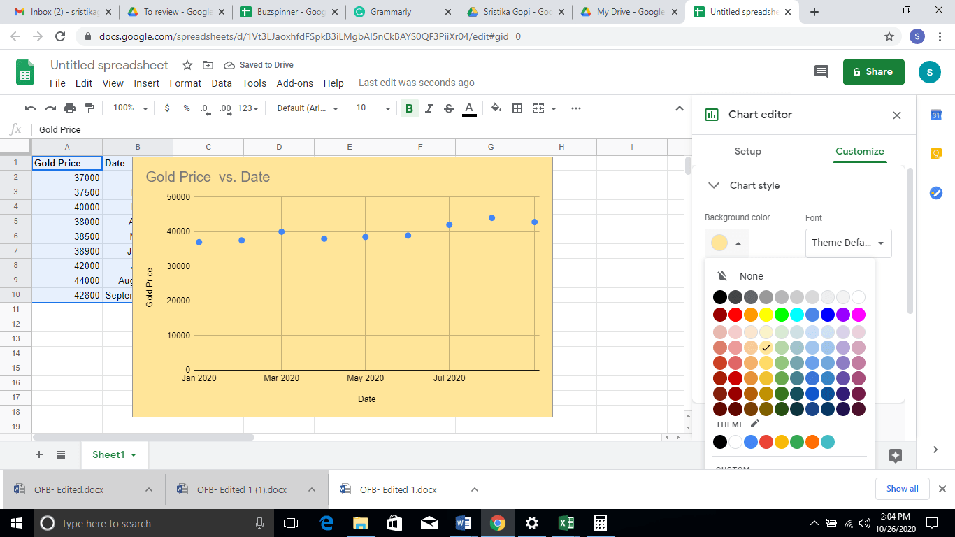
2. Click on the Chart Style, and you will see multiple options to change the style, such as color, background color, or new font style. Choose the background color and border color as per your preference.
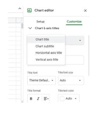
3. Click on the Charts and Axis titles and choose the dropdown Chart Title, you will four option where you can change Chart title, Chart subtitle, Horizontal axis title, and Vertical title. Choose the one for which you need to change the text.
   
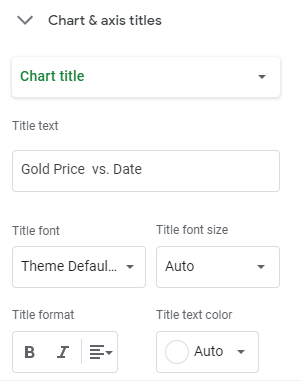
4. Give a new title in the Title Text Box, and you can also change the Title font and size by clicking the below option
   

Now, we have created the scatter plots and customized it. 

---

More about Customizing Scatter Plots

---

How to Make a Scatter Plot in Google Sheets with Trend line?

1. Navigate to the Customize tab and click on the Series option and then scroll down to click on the Trend line button 
2. On clicking the trend line button, you will be able to see the trend line displayed on your chart.
3. Click the customize option and change the Line Color, Type, and Label of the trend line.
   
   

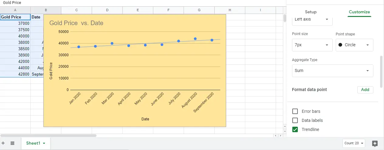
The below picture showcase how a linear trend line will look like on the scatter plot. If required, you can also resize the graph or change the elements as per the data set’s requirement.

Through this method, you can create a scatter plot with a trend line

How to Make a Scatter Plot in Google Sheets with Error Type?

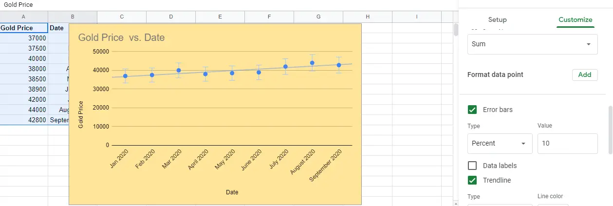
Similarly, you can also add Error Bars in the scatter plot graph. This will showcase how on-trend or reliable is the given data set. For instance, you can compare the retail price of the gold and display the over-priced retail location to help prospectus customers. 

You can add Error Bars in the scatter plot chart by following these steps:

1. Open your chart editor and click on the dots icon found at the right corner of your scatter plot. Select the “Edit chart” under the pop-up menu.
2. Select the “Customize” tab and expand the Series sub-section. Check the box against “Error bars” to include this feature in your scatter chart.
3. In your scatter plot graph, you will now see the error bars for every data point and represent how closely they are related to the trend line.

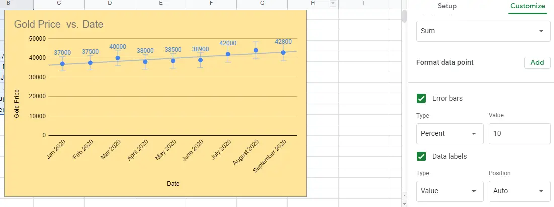
You can also get the data on each point, by clicking on the check box Data Labels

Similarly, you can customize the scatter plot further by clicking on the options like Gridlines and Ticks, Horizontal Axis, and Vertical Axis under the Customize tab 

I hope you find this post helpful and answer your question “How to Make a Scatter Plot In Google Sheets”